Machine Learning Tutorial #4: Creating the Timing Files
Overview
Once we have created a template, we will need to change the timings for each run. Each subject in the dataset has 12 timing files in their func folder, corresponding to each run of functional data. For example, the first few lines of the file sub-1_task_objectviewing_run-01_events.tsv in the folder sub-1/func looks like this:
onset   duration        trial_type
12.000  0.500   scissors
14.000  0.500   scissors
16.000  0.500   scissors
18.000  0.500   scissors
20.000  0.500   scissors
22.000  0.500   scissors
24.000  0.500   scissors
26.000  0.500   scissors
28.000  0.500   scissors
30.000  0.500   scissors
32.000  0.500   scissors
34.000  0.500   scissors
48.000  0.500   face
50.000  0.500   face
52.000  0.500   face
54.000  0.500   face
56.000  0.500   face
58.000  0.500   face
60.000  0.500   face
62.000  0.500   face
64.000  0.500   face
66.000  0.500   face
68.000  0.500   face
70.000  0.500   face
According to the Haxby et al. 2001 paper, each condition lasted for 24 seconds, and this is reflected in the Duration field that we specified in the last chapter. We will therefore need to extract the first onset time for each condition for each run, and concatenate them into a single timing file per condition. Later, we will use this timing file to fill in the remaining fields of our script.
The following code will extract the first onset time for each condition automatically, looping over all of the subjects in the dataset. You can either copy and paste this into the terminal, first making sure you are in the directory Haxby_Data that contains all of the subjects; else, you can copy it into a file, name it make_Timings.sh, and run it by typing bash make_Timings.sh:
#!/bin/bash
for subj in sub-1 sub-2 sub-3 sub-4 sub-5 sub-6; do
  cd ${subj}/func
    for cond in bottle cat chair face house scissors scrambledpix shoe; do
      if [ -f "$cond.txt" ]; then
        rm ${cond}.txt
      fi
          for i in `seq -w 1 12`; do
                  cat ${subj}_task-objectviewing_run-${i}_events.tsv | awk -v i="$cond" '{if ($3==i) print $1}' | head -1 >> ${cond}.txt
          done
    done
  cd ../..
done

(Note that errors for subject 5 run 12 are expected, and will be dealt with later.)
This will generate files labeled bottle.txt, cat.txt, and so on, one for each condition, and place it in the appropriate subject’s func folder. The contents of sub-1’s bottle.txt file, for example, will look like this:
228.000
192.000
156.000
228.000
84.000
228.000
264.000
156.000
228.000
264.000
120.000
12.000
Note that these onset times are relative to the start of each run. For example, the first value of 228.000 means that the “bottle” condition occurred 228 seconds into the first run; the next value indicates that 192.000 seconds into the second run was when the “bottle” condition was next presented; and so on.
Modifying the Script
In the previous chapter, we created a template script from the SPM GUI and labeled it Haxby_Script. This created two separate scripts, Haxby_Script_job.m which contains the SPM code that runs all of the commands specified in the GUI, and Haxby_Script.m, which contains the command spm_jobman which executes the file Haxby_Script_job.m. We will be editing the latter in order to read the timing files that we just created; to open it, from the Matlab terminal type open Haxby_Script_job.m (or click the Open button and select the script).
Note
This section draws upon many of the same principles discussed in the SPM chapter on scripting. If you haven’t already, it may help to work through the entire SPM tutorial in order to develop a foundation for what we will learn next.
Around line 58 is where the fMRI specification module is defined. Before the onset times are defined, enter the following code (I place this at lines 64-65 in my script):
load('sub-1/func/bottle.txt'); load('sub-1/func/cat.txt'); load('sub-1/func/chair.txt'); load('sub-1/func/face.txt');
load('sub-1/func/house.txt'); load('sub-1/func/scissors.txt'); load('sub-1/func/scrambledpix.txt'); load('sub-1/func/shoe.txt')
This will load each text file for sub-1 into a variable. Usually the variable is defined by typing something like x=load(bottle.txt), which assigns the values in bottle.txt to x. If no variable is defined on the left side of the equation, then the variable will default to the name of the text file that is loaded. In this case, the variables will be labeled bottle, cat, and so on.
Remember that when we created this script in the GUI, we left the onset times undefined. In the script, you will see the string <UNDEFINED> that was not filled in from the GUI; we will replace these with the appropriate values from the text files that we just loaded.
For example, the first onset field in my script is at line 67. Since this is the onset time for the bottle condition for run 1, I will need to extract the first row of the file bottle.txt. I can assign it to this field by replacing <UNDEFINED> with bottle(1,:). (You can double-check what value is being assigned by typing bottle(1,:) at the Matlab terminal.) We will then do this for the other conditions as well, which you can see in the figure below:
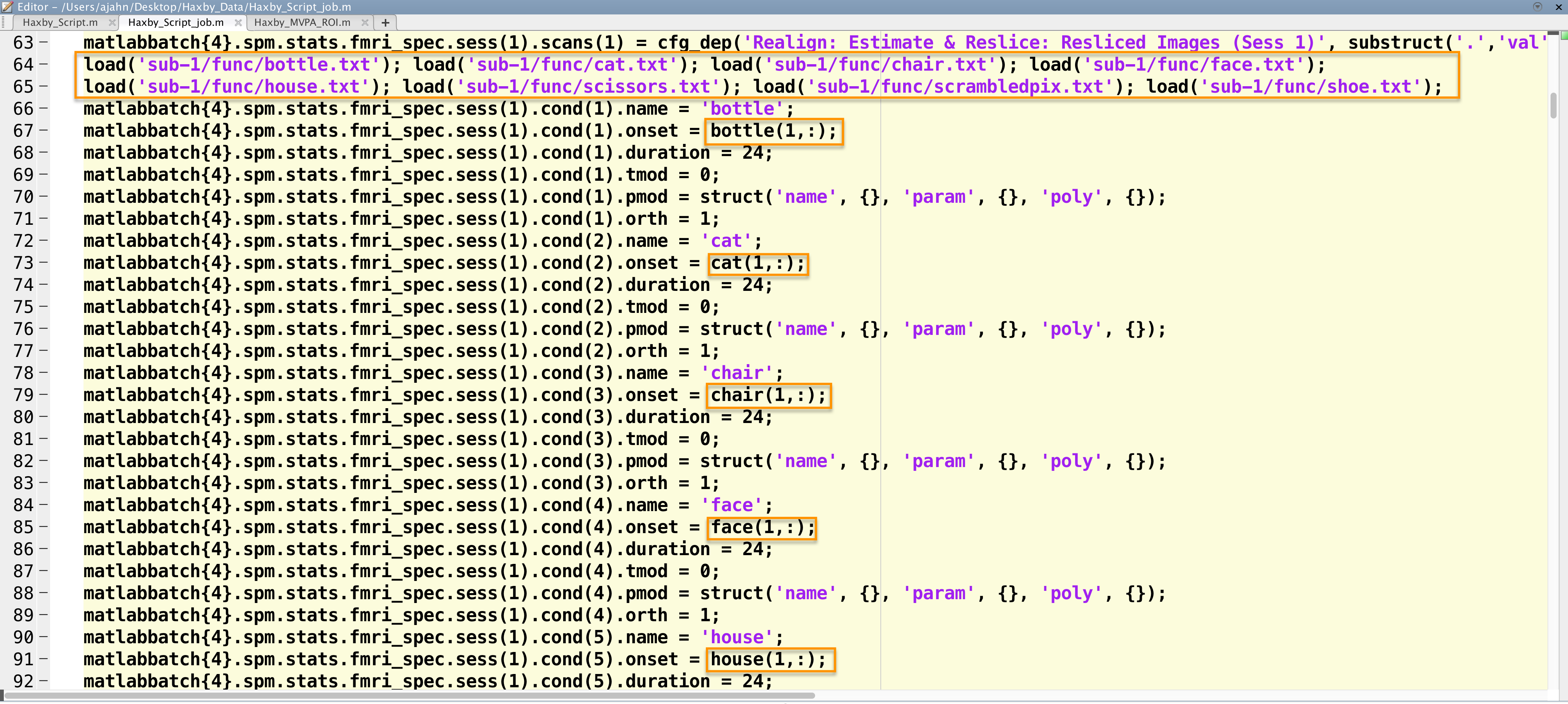
Snapshot of part of the script to analyze the Haxby dataset. The timing files are loaded, and then the appropriate line is extracted and inserted into the onset times field for each run.
These need to be replaced for each condition for the first run, and then done for each of the other runs. Again, this is tedious, but you will see that once we’ve done it once, with slight modifications we can run it for all of the other subjects. When we fill in the onset times for the other fields, we will need to extract the correct row; for the second run, for example, the code to extract the onset times for the bottle condition would be bottle(2,:).
Note
If you are uncertain about how to fill in the rest of the fields, a copy of the script can be downloaded here.
Lastly, add this line to the end of the script in order to run the code:
spm_jobman('run', matlabbatch)
And then run the script from the terminal by tying the name of the script:
Haxby_Script_job
It should take about an hour to run.
Video
For an overview of how to create the timing files for this study, click here.
Next Steps
When the script has finished, you should see a design matrix that looks like this:
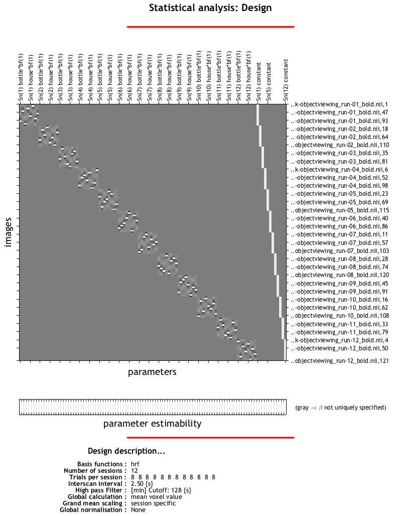
Each run should look like a separate square, with the tiny white squares within each run representing a block for each condition. Each of these blocks has been estimated as a separate beta map, which we will use as both training and testing data for our classifier. To learn how to do that, click the Next button.