fMRIPrep Tutorial #3: Examining the Preprocessed Data
Overview
When fMRIPrep has finished, the output will be located in the sub-directory derivatives/fmriprep. Within that directory, we see the folder sub-08; this contains all of the preprocessed functional and anatomical data, including intermediate files that were created in order to generate the final product, as well as “.json” files that contain header information for each of their corresponding images.
Within the anat directory, for example, we find the following files:
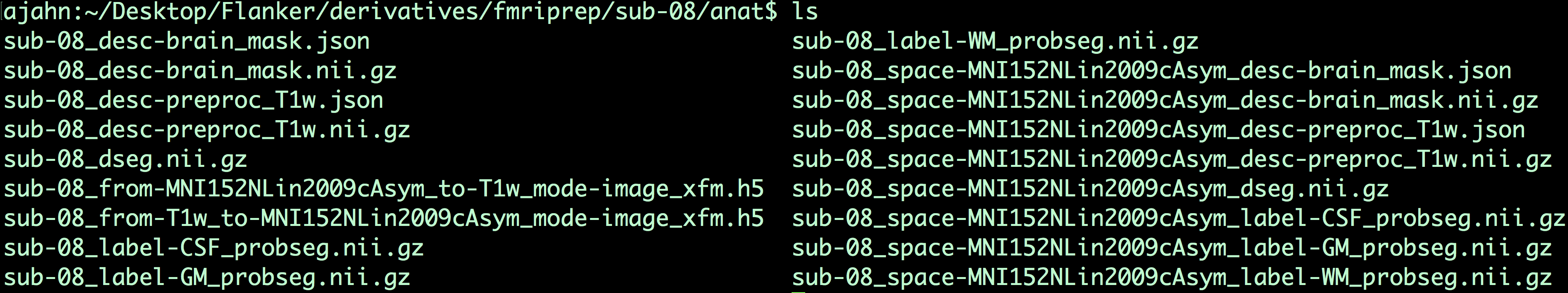
The files that contain the string MNI152NLin2009cAsym are anatomical images that have been normalized to that template, while those files without that string are in native space (i.e., they are not normalized). For example, the file sub-08_space-MNI152NLin2009cAsym_label-CSF_probseg.nii.gz is the CSF probabilistic segmentation in normalized space, while the anatomical image that has been preprocessed and normalized is the file sub-08_space-MNI152NLin2009cAsym_desc-preproc_T1w.nii.gz. Many of these files are intermediate images used to improve the normalization process, as well as for extracting the time-courses of tissue types as confound regressors.
Moving on to the func directory, we have the following:
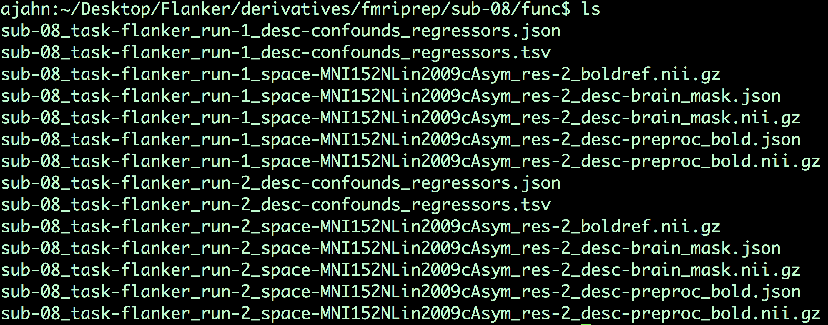
You will see two distinct blocks of files, one for each run. The first block contains a list of confound regressors, such as time-courses from the white matter and cerebrospinal fluid, and the motion parameters and their derivatives in the x-, y-, and z-directions. (For a review of motion parameters, see this chapter.) The file sub-08_task-flanker_run-1_space-MNI152NLin2009cAsym_res-2_boldref.nii.gz is the reference image used for registration and normalization, while the file sub-08_task-flanker_run-1_space-MNI152NLin2009cAsym_res-2_desc-brain_mask.nii.gz is the estimated brain mask for that run, and the file sub-08_task-flanker_run-1_space-MNI152NLin2009cAsym_res-2_desc-preproc_bold.nii.gz is the preprocessed functional data, up through normalization. Similar files are generated for the other runs in your dataset.
All of these output files will be used in the HTML summary, which we now turn to.
Note
Much of the QA analysis can be found here on the fMRIPrep ReadTheDocs webpage. The following recapitulates most of what is on that site, applied to the current dataset.
The HTML Output
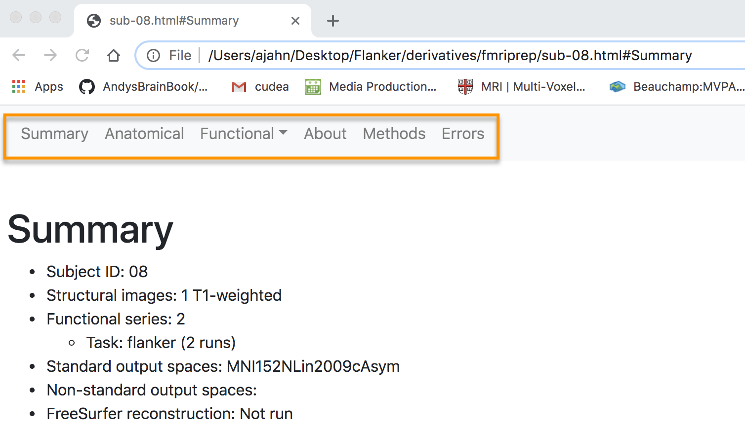
fMRIPrep summarizes all of the preprocessing output in a single HTML file called sub-08.html. You can open this by using finder and double-clicking on the file, or navigating to the directory with your terminal and typing open sub-08.html.
The layout of the webpage is organized into the following sections: Summary, Anatomical, Functional, About, Methods, and Errors, with corresponding links at the top of the page. The first section, “Summary”, contains details about the number of structural and functional images, the template that was used for normalization, and whether FreeSurfer was run. These should match the options you specified in the fmriprep.sh script that we ran in the previous chapter
Although the output of fMRIPrep in the terminal should note whether there were any errors during preprocessing, it’s worth checking the Error tab first to see whether there is anything that you need to address.
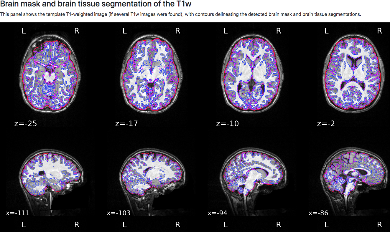
Anatomical QA
The next section contains anatomical QA checks, with the first figure showing the anatomical image in sagittal, axial, and coronal views. The estimated brain mask is outlined in red, the grey matter boundary is outlined in magenta, and the white matter boundary is outlined in blue. These boundaries will be used for component extraction, which is discussed in more detail below.
Normalization of the anatomical image to the template - in this case, the MNI152NLin2009cAsym template - is shown in a back-and-forth GIF. Make sure to check the alignment not only between the outlines of the brain, but also the internal structures such as the ventricles:
Functional QA
We now move on to the functional QA, which uses a GIF to show the alignment between the functional and anatomical images. As with the normalization QA check, make sure that the internal structures are well aligned, remembering that lighter voxels in the functional images represent fluid, and vice versa in the anatomical image:
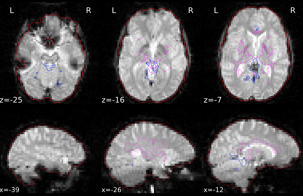
The next figure shows an outline of the masks used for anatomical component correction (anatCompCor), with magenta showing the white matter and CSF voxels used to estimate signal that is representative of that area. The voxels outlined in blue show the most variable voxels, which will be used for functional component correction (funcCompCor):
These voxels are then used to generate compCor curves for the white matter, CSF, combined white matter and CSF, and temporal standard deviation, which show the amount of variance explained by different amounts of components. The first 27 components of the white matter mask, for example, explain half of the variance within those voxels; you will have to make a judgment about the tradeoff between removing nuisance variance, and spending more degrees of freedom and statistical power on modeling those sources of variance.

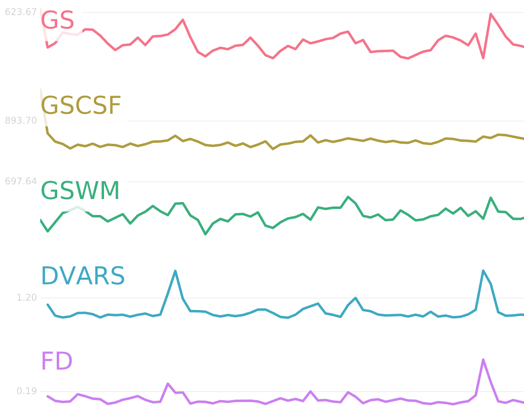
Time-series plots are also generated for global signal (GS), global signal of the cerebrospinal fluid (GSCSF), global signal of the white matter (GSWM), and two measures of motion: DVARS and Framewise Displacement (FD). Changes in motion tend to be correlated with changes in global signal, and it is up to you whether to include any of these regressors in your model. In general, DVARS and FD are good ways to account for signal caused by motion artifacts.
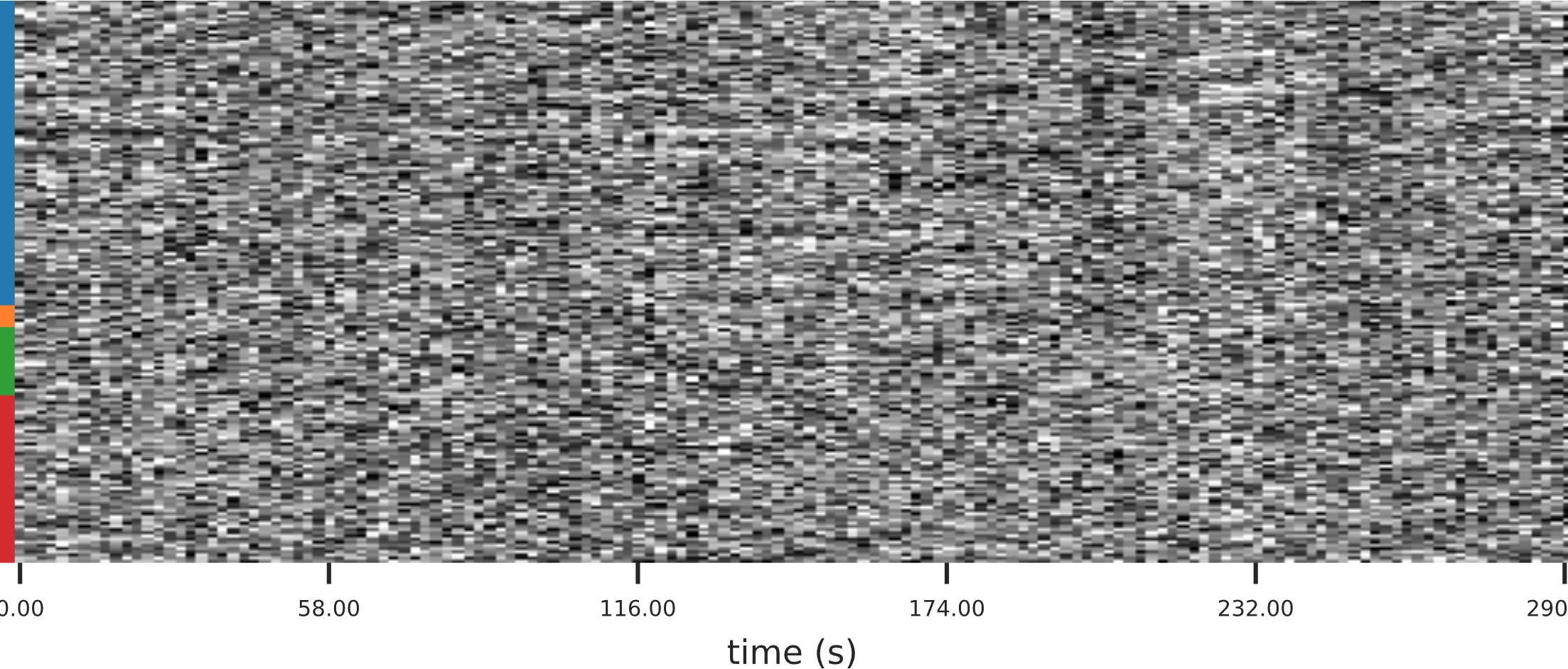
The next figure is a carpet plot, showing the time-series of each major tissue type. Voxels are grouped into cortical (dark/light blue), and subcortical (orange) gray matter, cerebellum (green) and white matter and CSF (red). Any sudden changes in motion may be reflected in uniform changes across the entire column for that timepoint.
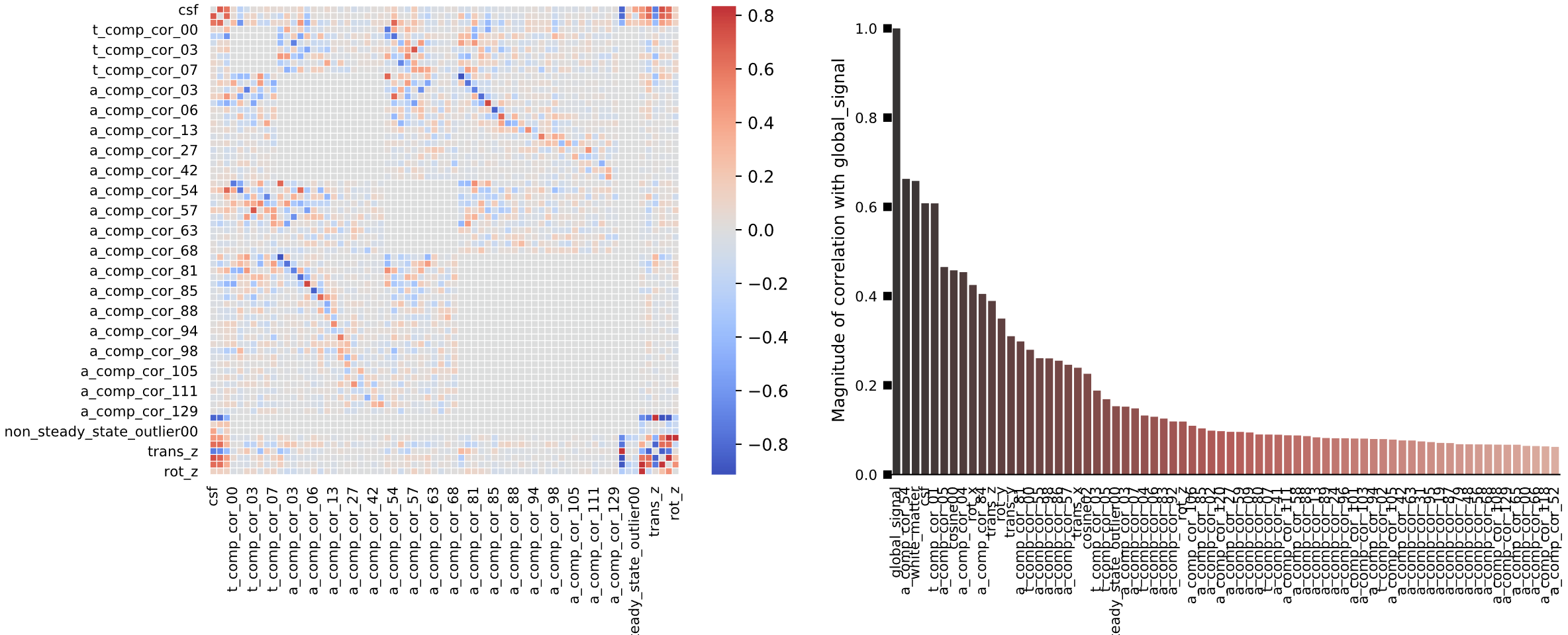
Lastly, a matrix shows correlations between the different nuisance regressors. High correlation between the CSF regressor and the trans_z and rot_z motion regressors, for example, may be explained by motion causing signal changes in the CSF that encases the skull. The bar chart on the right shows the correlation of different regressors with respect to global signal; those components that show a high degree of correlation may be candidates for nuisance regression.
Next Steps
Now that we have run quality checks on our data and have some idea of what regressors to include, we are prepared to begin creating our general linear model. Before we can do that, however, we have the option of running a couple more preprocessing steps. To see what those are and how to do them, click the Next button.
Video
For a video demonstration of QA checks with fMRIPrep, click here.