MRtrix Tutorial #6: Creating the Tissue Boundaries
We are almost ready to begin our streamline analysis, in which we will place seeds at random locations along the boundary between the grey matter and the white matter. A streamline will grow from each seed and trace a path from that seed region until it terminates in another region. Some of the streamlines will terminate in places that don’t make sense - for example, a streamline may terminate at the border of the ventricles. We will cull these “error” streamlines, and be left with a majority of streamlines that appear to connect distant grey matter regions.
To do this, we will first need to create a boundary between the grey matter and the white matter. The MRtrix command 5ttgen will use FSL’s FAST, along with other commands, to segment the anatomical image into five tissue types:
- Grey Matter;
- Subcortical Grey Matter (such as the amygdala and basal ganglia);
- White Matter;
- Cerebrospinal Fluid; and
- Pathological Tissue.
Once we have segmented the brain into those tissue classes, we can then use the boundary as a mask to restrict where we will place our seeds.
Converting the Anatomical Image
The anatomical image first needs to be converted to MRtrix format. Just as we did in a previous chapter, we will use the command mrconvert. If you are in the dwi directory, you can type the following:
mrconvert ../anat/sub-CON02_ses-preop_T1w.nii.gz T1.mif
This creates a new file, T1.mif, which you can look at in mrview.
We will now use the command 5ttgen to segment the anatomical image into the tissue types listed above:
5ttgen fsl T1.mif 5tt_nocoreg.mif
This command will take about 10-15 minutes. If the segmentation has finished successfully, you should see the following images when you type mrview 5tt_nocoreg.mif (pressing the left and right arrow keys scrolls through the different tissue types):
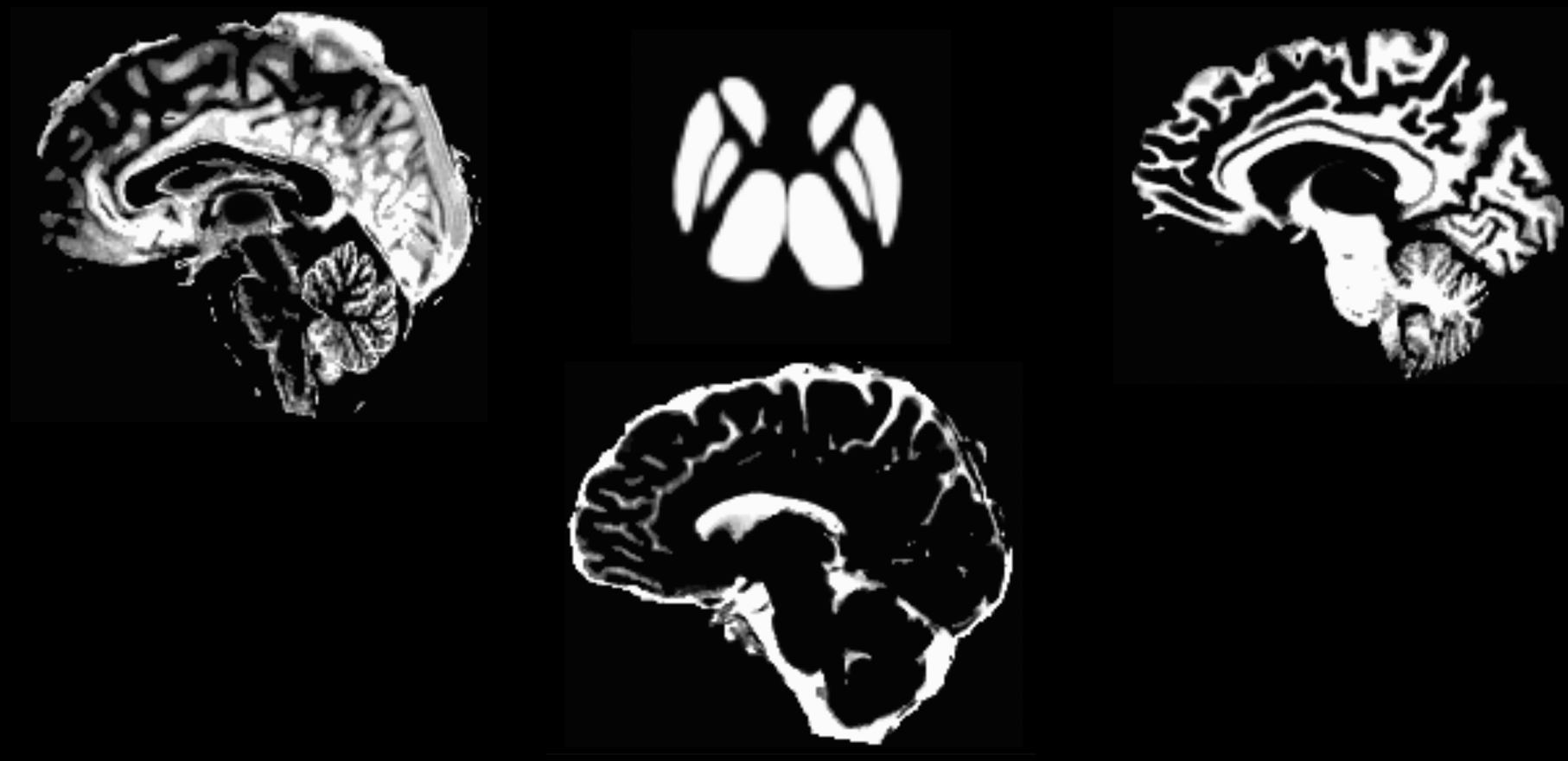
The output from 5ttgen fsl anat.mif 5tt_nocoreg.mif will be a single dataset with 5 volumes, one per tissue type. Check this image with mrview, using the right and left arrow keys to toggle between tissue types. The tissue types are: GM, WM, CSF, subcortical GM, and pathological tissue. If no pathological tissue is detected, then that volume is blank.
Note
If the segmentation step fails, this may be due to insufficient contrast between the tissue types; for example, some anatomical images are either very dark across both the grey and white matter, or very light across both tissue types. We can help the segmentation process by increasing the intensity contrast (also known as intensity normalization) between the tissues with a command like AFNI’s 3dUnifize, e.g.:
3dUnifize -input anat.nii -prefix anat_unifize.nii
The difference between the image before and after may be subtle, but it can prevent a segmentation error from being thrown.
Coregistering the Diffusion and Anatomical Images
If the segmentation has finished without any errors, our next step is to coregister the anatomical and diffusion-weighted images. This ensures that the boundaries of the tissue types are aligned with the boundaries of the diffusion-weighted images; even small differences in the location of the two scans can throw off the tractography results.
We will first use the commands dwiextract and mrmath to average together the B0 images from the diffusion data. These are the images that look most like T2-weighted functional scans, since a diffusion gradient wasn’t applied during their acquisition - in other words, they were acquired with a b-value of zero. To see how this works, navigate back to the dwi directory and type the following command:
dwiextract sub-02_den_preproc_unbiased.mif - -bzero | mrmath - mean mean_b0.mif -axis 3
There are two parts to this command, separated by a pipe (”|”). The left half of the command, dwiextract, takes the preprocessed diffusion-weighted image as an input, and the -bzero option extracts the B0 images; the solitary - argument indicates that the output should be used as input for the second part of the command, to the right of the pipe. mrmath then takes these output B0 images and computes the mean along the 3rd axis, or the time dimension. In other words, if we start with an index of 0, then the number 3 indicates the 4th dimension, which simply means to average over all of the volumes.
In order to carry out the coregistration between the diffusion and anatomical images, we will need to take a brief detour outside of MRtrix. The software package doesn’t have a coregistration command in its library, so we will need to use another software package’s commands instead. Although you can choose any one you want, we will focus here on FSL’s flirt command.
The first step is to convert both the segmented anatomical image and the B0 images we just extracted:
mv ../anat/5tt_nocoreg.mif .
mrconvert mean_b0.mif mean_b0.nii.gz
mrconvert 5tt_nocoreg.mif 5tt_nocoreg.nii.gz
Since flirt can only work with a single 3D image (not 4D datasets), we will use fslroi to extract the first volume of the segmented dataset, which corresponds to the Grey Matter segmentation:
fslroi 5tt_nocoreg.nii.gz 5tt_vol0.nii.gz 0 1
We then use the flirt command to coregister the two datasets:
flirt -in mean_b0.nii.gz -ref 5tt_vol0.nii.gz -interp nearestneighbour -dof 6 -omat diff2struct_fsl.mat
This command uses the grey matter segmentation (i.e., “5tt_vol0.nii.gz”) as the reference image, meaning that it stays stationary. The averaged B0 images are then moved to find the best fit with the grey matter segmentation. The output of this command, “diff2struct_fsl.mat”, contains the transformation matrix that was used to overlay the diffusion image on top of the grey matter segmentation.
Now that we have generated our transformation matrix, we will need to convert it into a format that can be read by MRtrix. That is, we are now ready to travel back into MRtrix after briefly stepping outside of it. The command transformconvert does this:
transformconvert diff2struct_fsl.mat mean_b0.nii.gz 5tt_nocoreg.nii.gz flirt_import diff2struct_mrtrix.txt
Note that the above steps used the anatomical segmentation as the reference image. We did this because usually the coregistration is more accurate if the reference image has higher spatial resolution and sharper distinction between the tissue types. However, we also want to introduce as few edits and interpolations to the functional data as possible during preprocessing. Therefore, since we already have the steps to transform the diffusion image to the anatomical image, we can take the inverse of the transformation matrix to do the opposite - i.e., coregister the anatomical image to the diffusion image:
mrtransform 5tt_nocoreg.mif -linear diff2struct_mrtrix.txt -inverse 5tt_coreg.mif
The resulting file, “5tt_coreg.mif”, can be loaded into mrview in order to examine the quality of the coregistration:
mrview sub-02_den_preproc_unbiased.mif -overlay.load 5tt_nocoreg.mif -overlay.colourmap 2 -overlay.load 5tt_coreg.mif -overlay.colourmap 1
The “overlay.colourmap” options specify different color codes for each image that is loaded. In this case, the boundaries before coregistration will be depicted in blue, and the boundaries after coregistration will be shown in red:
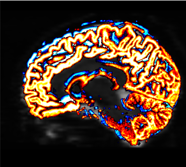
The change in the boundaries before and after coregistration may be very slight, but they will have a large effect on the rest of the steps that we do. Make sure to check the boundaries in all three views; you can also use the Tool -> Overlay menu to display or hide the different overlays.
The last step to create the “seed” boundary - the boundary separating the grey from the white matter, which we will use to create the seeds for our streamlines - is created with the command 5tt2gmwmi (which stands for “5 Tissue Type (segmentation) to Grey Matter / White Matter Interface)
5tt2gmwmi 5tt_coreg.mif gmwmSeed_coreg.mif
Again, we will check the result with mrview to make sure the interface is where we think it should be:
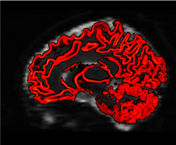
mrview sub-02_den_preproc_unbiased.mif -overlay.load gmwmSeed_coreg.mif
You should see something like this at the end:
Next Steps
Now that we have determined where the boundary is between the grey matter and the white matter, we are ready to begin generating streamlines in order to reconstruct the major white matter pathways of the brain. We will see how to do that in the next chapter.