Chapter #11: Task-Related Connectivity and gPPI

---

Overview

Until now, we have analyzed resting-state data, in which the subject does nothing except remain still and awake. However, it is also common for studies to collect task-related data as well, in which the subject does some kind of activity; such as doing the Flanker Task, for example. In this chapter we will cover how to analyze task-related data by using a technique called Psychophysiological Interactions (PPI), which reveals whether the functional connectivity between two nodes depends on what task the subject is currently doing.

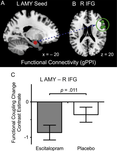
Example of a PPI analysis, taken from Outhred et al. (2015). The functional connectivity between the left amygdala seed region and the right IFG changes depending on which condition the subject is in.

Traditional PPIs

Originally, a psychophysiological interaction consisted of modeling three terms (Friston, 1997):

1. A task regressor indicating which of two tasks the subject was currently doing;

2. A time-series regressor extracted from a seed region; and

3. An interaction term, consisting of the product of the task regressor multiplied by the time-series regressor.

The interaction term was then tested for significance. In other words, a significant voxel would show differences in functional connectivity as a function of task. The figure below shows how these regressors are constructed:

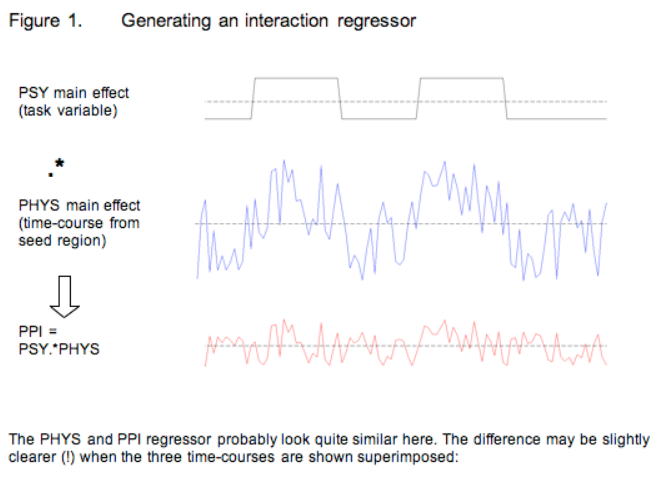
An illustration of PPI regressors. The top panel shows a binary regressor composed of 1’s and -1’s, indicating whether the subject is in one of two conditions. The middle panel shows a time-series extracted from a seed region. The bottom panel shows the interaction regressor, created by multiplying the above regressors. Note how the -1’s, when multiplied by the seed time-series, invert the sign of the time-series - if the time-series is going down, in the interaction regressor it will go up.

The interaction regressor is then compared against the time-series of every other voxel in the brain. If there is a good correspondence between the two, the significance of the fit is higher. Both figures are taken from the FSL website.

Generalized PPIs

A more recent version of PPI is known as generalized PPI (gPPI) (McLaren et al., 2012). This method creates a PPI term for each condition in the study, in addition to the regressor of the seed time-series and individual regressors for each condition. If the study has N conditions, then the gPPI analysis will contain 2N+1 regressors.

As an example, let’s say that we have three conditions in our experiment: A, B, and C. The gPPI analysis would consist of the following regressors:

1. Regressor for A

2. Regressor for B

3. Regressor for C

4. Time-series regressor for the seed region

5. PPI for A

6. PPI for B

7. PPI for C

Even if one of these conditions is of no interest, modeling the entire experimental space will be more accurate than restricting the PPI to only a pair of the regressors.

Setting up a gPPI in the CONN Toolbox

So far, we have used the CONN toolbox to model one condition: The resting-state condition, which is simply the time-series at each of our ROIs that we have selected in the Setup tab. We will now load a separate scan that was collected while the subject was doing a task, and which has two conditions: The main task, in which the subject was doing an arithmetic problem, and a control task, in which the subject was doing nothing. The onset times for each of these conditions can be found in the “events.tsv” files on the openneuro webpage for the Arithmetic dataset.

subjects = [01 02 03 04 05 06];

for subject=subjects

  subject=num2str(subject, '%02d');
  movefile(['~/Downloads/sub-' num2str(subject) '_func_sub-' num2str(subject) '_task-arithm_run-01_bold.nii.gz'], ['sub-' num2str(subject) '/func'])
  movefile(['~/Downloads/sub-' num2str(subject) '_func_sub-' num2str(subject) '_task-arithm_run-02_bold.nii.gz'], ['sub-' num2str(subject) '/func'])
  movefile(['~/Downloads/sub-' num2str(subject) '_func_sub-' num2str(subject) '_task-arithm_run-01_events.tsv'], ['sub-' num2str(subject) '/func'])
  movefile(['~/Downloads/sub-' num2str(subject) '_func_sub-' num2str(subject) '_task-arithm_run-02_events.tsv'], ['sub-' num2str(subject) '/func'])

end

Note

To review onset times, and how they are used to construct a general linear model, see this module.

We will first demonstrate this with a single subject, and then with a group analysis. Go back to the Setup tab, and click on “Basic”. Set the number of subjects to “1”, and the CONN toolbox will ask which subjects you want to delete. Hold down shift and click to select subjects 2-6, so that only subject 1 remains. Click on the “Functional” button, and select the file sub-01_func_sub-01_task-arithm_run-01_bold.nii.gz. This will replace the resting-state scan with a task-related scan.

Then, click on the “Conditions” tab. Clicking on the New sign when you hover over the Conditions column will allow you to specify a new regressor. In the “Condition name” field, type control_condition, and click on the dropdown menu below “Condition definition” to select “task designs: condition present at blocks/events during selected session(s)”. This will generate two new fields, “Onset” and “Duration”, which you can use to specify when the condition happened, and for how long. Looking at the .tsv file, we see that the onsets were 21.5, 63.5, 105.5, and so on, while the durations were 18.5 for each event. Type the onsets and the durations for each occurrence of the control condition, and then press enter. You can then do the same for the other condition, which we will call main_condition.

Doing this once can be a useful exercise, but you most likely will not want to do this for large numbers of subjects. A better alternative is to load the .tsv files through the CONN GUI automatically, which will fill in all of the fields for you. Highlight the conditions you just created and click the x sign to remove them, and then click on the - condition tools: dropdown menu and select import condition info from text file(s). Since this data is in BIDS format, we can select the option BIDS-compatible. (You can select either option for the single subject; when you have more sessions and more subjects, you will want to select the option “one *_events.tsv file in each subject/session folder.) When the onset files are loaded, you will see the following figure in the Study Design window:

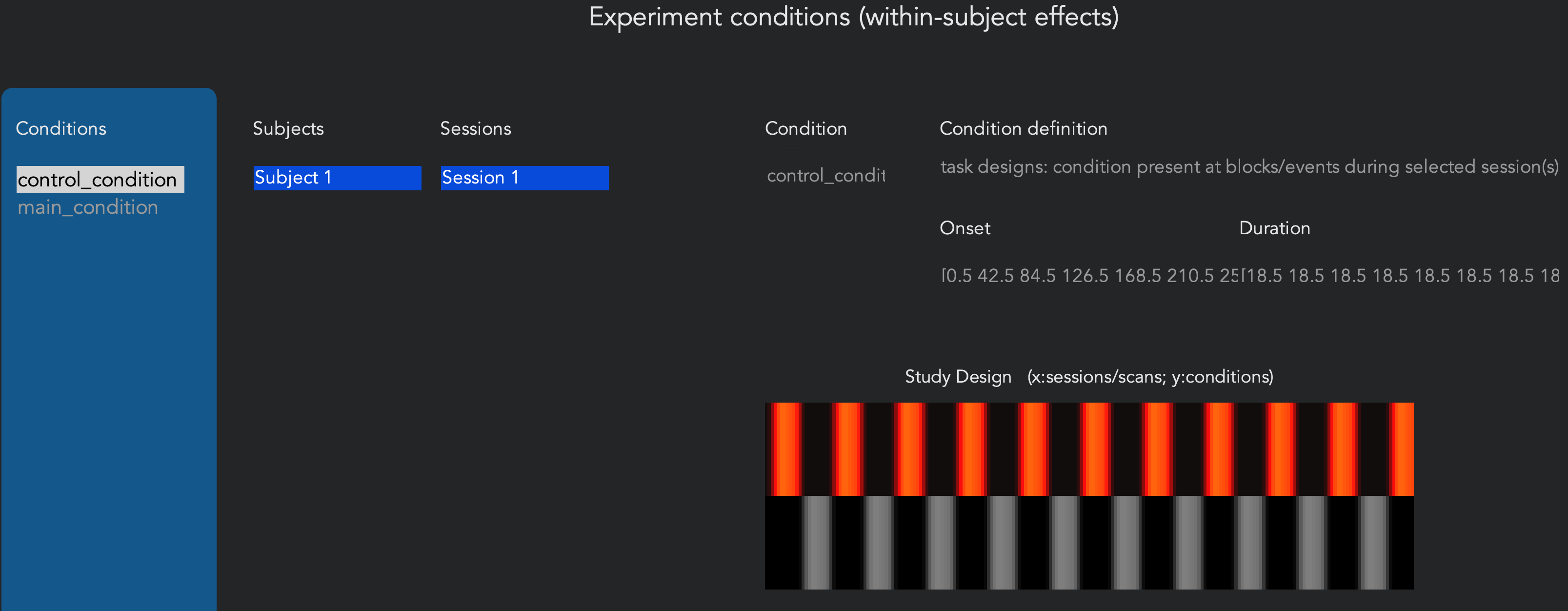
The study design window. Bars indicate the onset and duration of each trial, with separate conditions on each row. Highlighted bars reflect the condition and session that is currently selected in the left-hand menus.

When you are finished importing the timing files, click OK. Just as with the functional connectivity analysis, you will need to then run preprocessing, Setup, and Denoising, using similar QA checks.

Viewing the Results

After you’ve done preprocessing, Setup, and Denoising, you will have access to the 1st-level tab. The procedure is similar to what we did with the correlation analysis, but we will make the following changes:

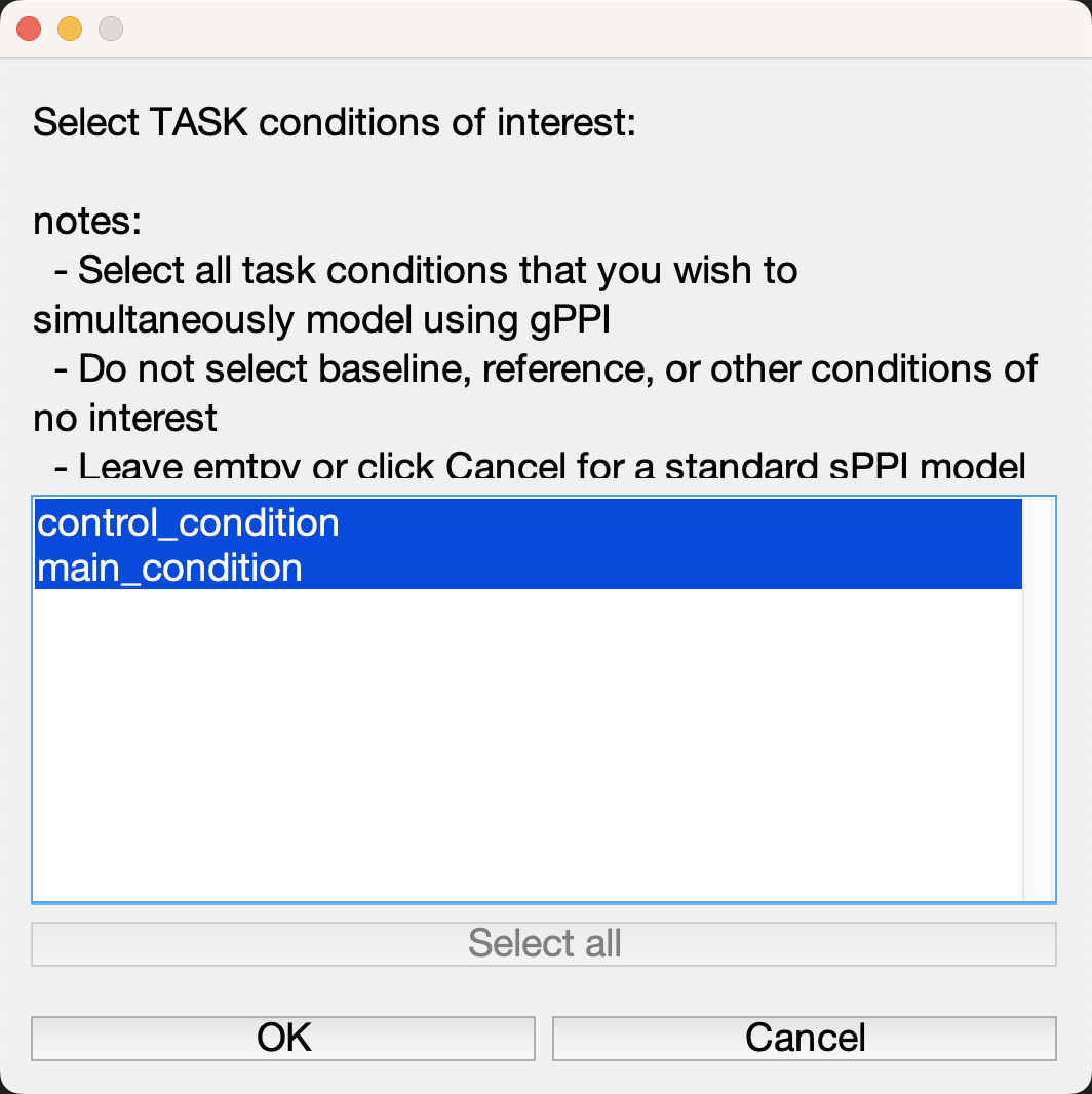
1. Click on the new button at the bottom of the Analyses panel on the left, and change the analysis type to gPPI (task-based generalized psychophysiological interactions), which will prompt you to select all of your task conditions of interest. Remember that we want to model the entire experimental space; in this case, we will select both and click OK. When it prompts you to “Save these changes to the CONN project?”, select Now.

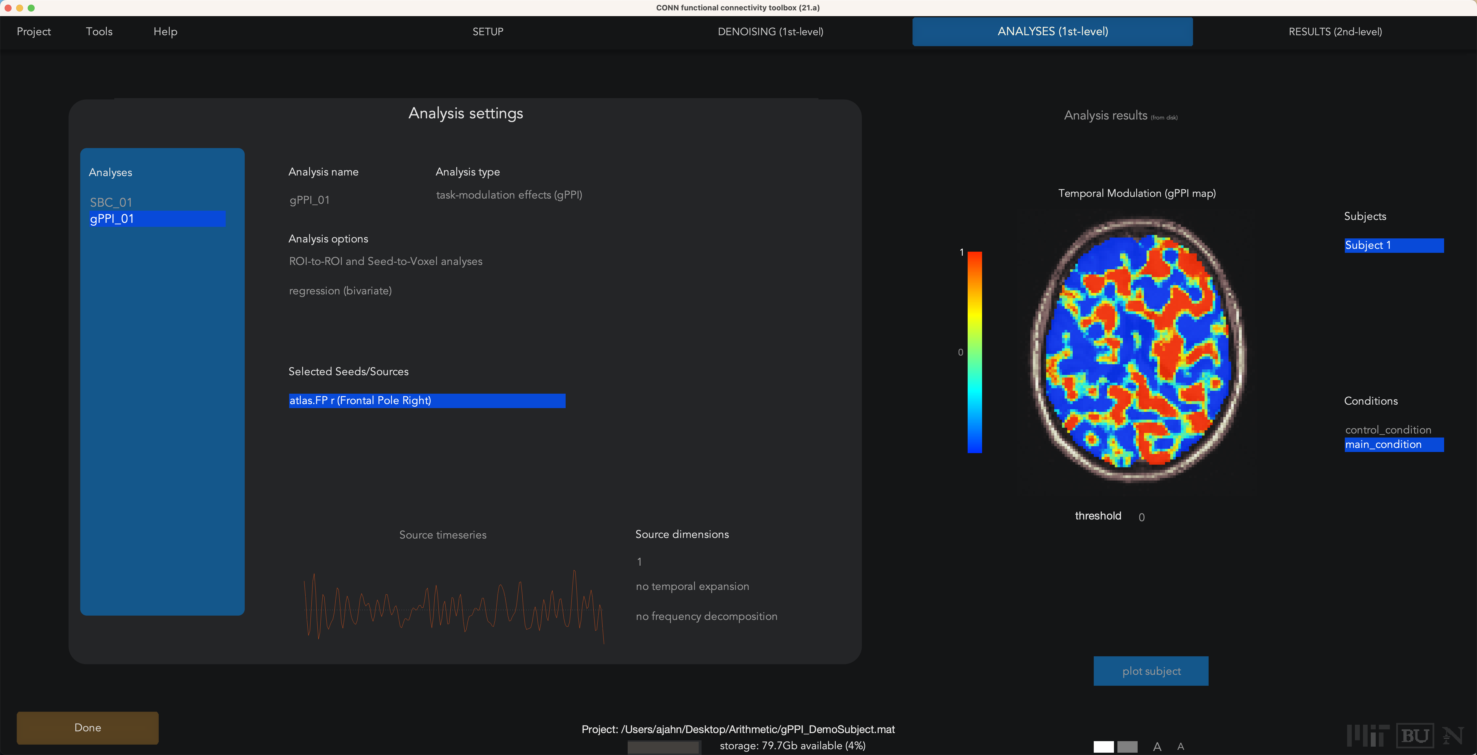
2. The other change is to switch the analysis options from correlation to regression (bivariate). Notice that once you run the 1st-level analysis, the values in the preview window are not correlation coefficients anymore; they are beta weights for the interaction term. For example, if we have the right Frontal Pole region highlighted and we switch to main_condition, the map shows which voxels are significantly more correlated with the right frontal pole during the main_condition.

Note

Before going on, think about this: With the functional connectivity analyses, one of our QA checks was whether the currently highlighted seed region was most significantly correlated with itself, which made sense. Here, if we set the threshold to only show the highest beta weights, there doesn’t seem to be much of anything in that seed region. Given what you just learned about gPPI, why do you think that is?

For the next step, click on the Done button. This will run a gPPI using all of the seed regions that are in the lefthand menu. If you have an hypothesis about one or two regions, you would only select those, and remove everything else. In this case, let’s just leave in the left and right frontal pole, and then click Done. This will take about a minute to run.

The second-level tab will be the same as what we saw in the video about viewing results. This study wasn’t designed for a gPPI analysis, and PPI effects are notoriously difficult to find in any case; so it isn’t surprising that we don’t see anything here. Nevertheless, if you did find an effect, you would need to follow the same steps of correcting for type 1 errors.

Generalized Functional Connectivity

Including task regressors also creates the possibility of doing Generalized Functional Connectivity, a method of generating resting-state functional connectivity maps from task-based datasets. This method, developed by Elliott et al. (2019), regresses out any effects of task and other nuisance covariates (for example, the usual ones of motion and physiological regressors), and creates functional connectivity maps of the remaining variance. According to Elliott et al., connectivity maps generated this way can lead to test-retest reliability that is comparable to functional data that was collected solely for resting-state, without any task conditions.

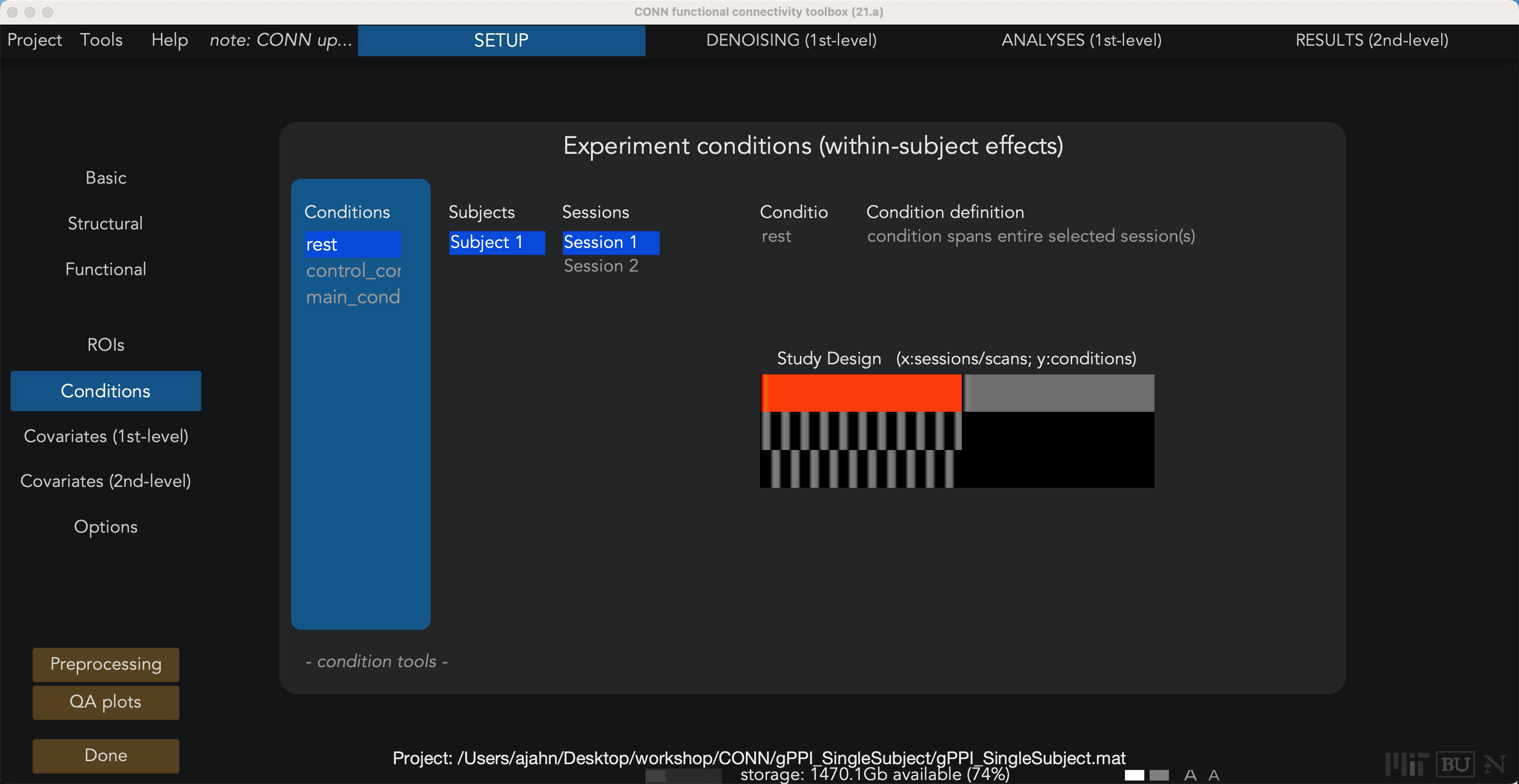
Furthermore, this method can theoretically increase your power by allowing you to combine both resting-state runs and data from task-based runs. Taking one resting-state and one task-based dataset from our current example, you should first preprocess them both separately (using the “Session” selector in the Preprocessing window if needed). After preprocessing, click on the Conditions button, and load any task regressors for the task-based run. Both runs should contain a regressor called “rest”, as seen below:

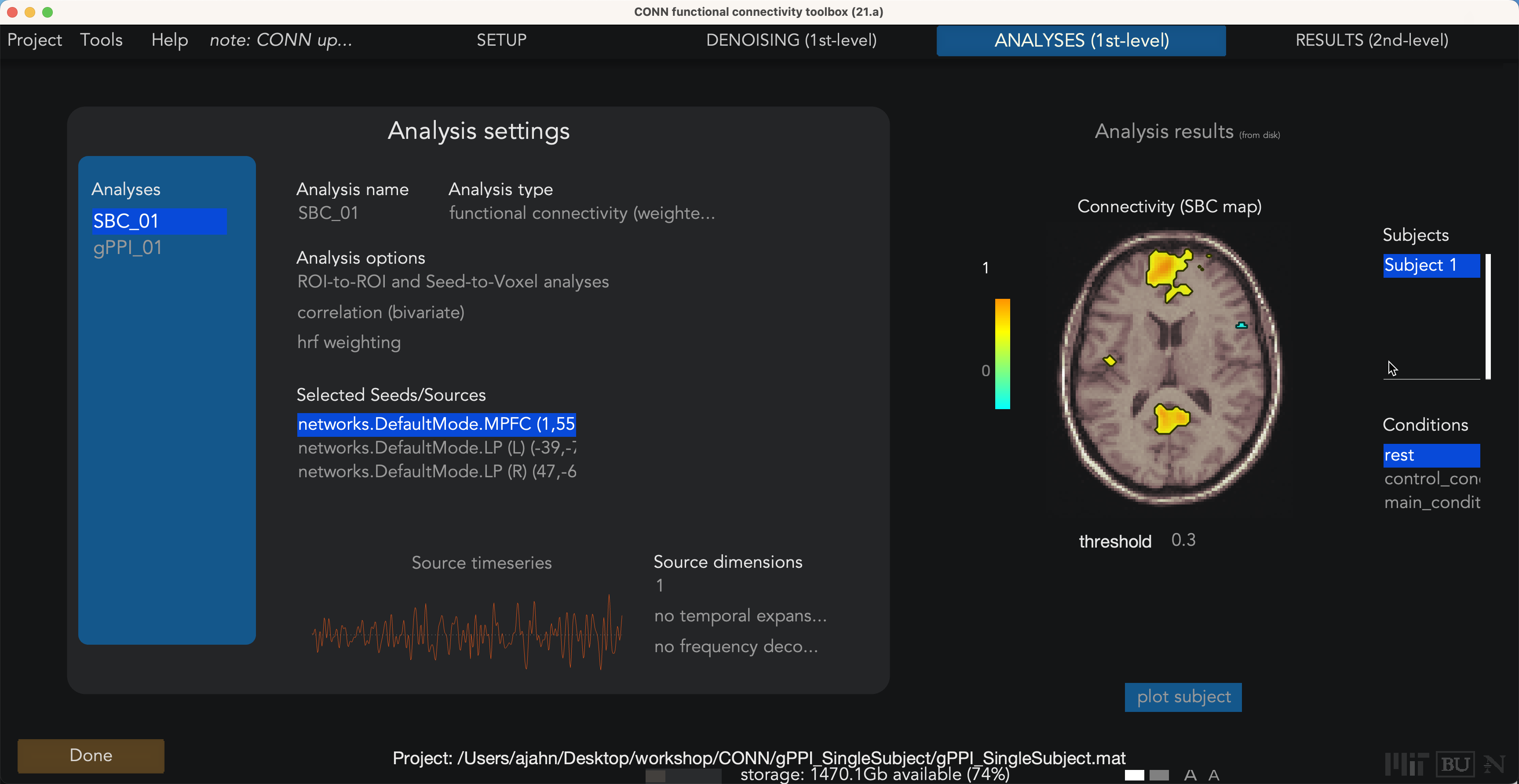
Do the denoising as usual, and then when you get the 1st-level tab and analyze the ROIs you are interested in, you should see something like this, which seems to be an average of the “rest” regressor over both sessions:

The only issue that can come up is if the TRs for the resting-state and task-based data are different; in that case, see this thread for potential ways to address that problem.

Next Steps

In this tutorial, we briefly touched on how automating the loading of onset data can save you time. In the next and last tutorial, we will learn how to automate our entire analysis by using something called scripting. To find out how to do it, click the Next button.

Video

A video overview of how to do gPPIs, including loading onset times, can be found here.